library(knitr)
library(kableExtra)
library(brms)
library(dplyr, warn.conflicts = FALSE)
#install.packages("dendextend")
#install.packages("circlize")
library(dendextend)
library(circlize)
library(digest)
# install.packages("cmdstanr", repos = c("https://mc-stan.org/r-packages/", getOption("repos")))
library(cmdstanr)
# install_cmdstan()
library(Matrix)
library(tidyverse)
library(reactable)
library(htmltools)
# install.packages("dendsort")
library(dendsort)
library(ggplot2)
library(ggdendro)
require(gridExtra)
# install.packages("ggplot2")
# library(ggplot)
# devtools::install_github("NightingaleHealth/ggforestplot")
# library(ggforestplot)epilepsy
Code (scroll past)
families = list(
  poisson=poisson(), negbinomial=negbinomial()
)
build_full_df <- function(model_df){
build_formula_string <- function(row){
rv = "count ~"
uterms = c("1")
for(col in names(model_df)[2:length(model_df)]){
what = row[col]
if(what != ""){
uterms = c(uterms, what)
}
}
paste(rv, paste(uterms, collapse="+"))
}
build_formula <- function(row){
# brmsformula(as.formula(build_formula_string(row)), family=families[[row["family"]]])
brmsformula(as.formula(build_formula_string(row)), family=row["family"])
}
build_name <- function(row){
paste0(row[["family"]], "(", build_formula_string(row), ")")
}
build_fit <- function(row){
brm(
build_formula(row),
data=epilepsy,
file=digest(build_name(row), algo="md5"),
backend="cmdstanr", silent=2, refresh=0
)
}
build_loo <- function(row){
# print(build_name(row))
file_name = paste0(digest(build_name(row), algo="md5"), "_loo.rds")
if(file.exists(file_name)){
return(readRDS(file_name))
}else{
rv = loo(build_fit(row), model_names=c(build_name(row)))
saveRDS(rv, file_name)
return(rv)
}
}
model_names = apply(model_df, 1, build_name)
rownames(model_df) <- model_names
loos = apply(model_df, 1, build_loo)
comparison_df = loo_compare(loos)
pbma_weights = loo_model_weights(loos, method="pseudobma")
pbma_df = data.frame(pbma_weight=as.numeric(pbma_weights), row.names=names(pbma_weights))
full_df = merge(model_df, comparison_df, by=0)
rownames(full_df) <- full_df$Row.names
full_df = full_df[2:length(full_df)]
full_df = merge(full_df, pbma_df, by=0)
rownames(full_df) <- full_df$Row.names
full_df = full_df[2:length(full_df)]
treatment_sampless = apply(full_df, 1, function(row){
if(row["Trt"] == ""){
return(c(0., 0.))
}
return(posterior_samples(build_fit(row))$b_Trt)
})
full_df = cbind(full_df,
model_name=model_names,
treatment_mean=as.numeric(lapply(treatment_sampless, mean)),
treatment_se=as.numeric(lapply(treatment_sampless, sd)),
treatment_q05=as.numeric(lapply(treatment_sampless, partial(quantile, probs=.05, names=FALSE))),
treatment_q25=as.numeric(lapply(treatment_sampless, partial(quantile, probs=.25, names=FALSE))),
treatment_q75=as.numeric(lapply(treatment_sampless, partial(quantile, probs=.75, names=FALSE))),
treatment_q95=as.numeric(lapply(treatment_sampless, partial(quantile, probs=.95, names=FALSE)))
)
return(full_df)
}
build_distancess <- function(model_df, df_, col_){
full_df = build_full_df(model_df)
scale = max(df_[[col_]]) - min(df_[[col_]])
build_distances <- function(row1){
build_distance <- function(row2){
rv = 0
for(col in names(model_df)){
rv = rv + (row1[col] != row2[col])
}
rv = rv + abs((as.numeric(row1[col_]) - as.numeric(row2[col_]))/scale)
rv
}
apply(df_, 1, build_distance)
}
distances = apply(df_, 1, build_distances)
rownames(distances) <- rownames(full_df)
colnames(distances) <- rownames(full_df)
return(distances)
}
build_color <- function(row){
rgb(0., 0., 0., as.numeric(row[["pbma_weight"]]))
# rgb(0., 0., 0., .1 + .9 * as.numeric(row[["pbma_weight"]]))
}
dendrogram_plot <- function(model_df, col_){
full_df = build_full_df(model_df)
distances = build_distancess(model_df, full_df, col_)
hc <- dendsort(as.dendrogram(hclust(as.dist(distances))))
hc_df = full_df[hc %>% labels,]
pbma_weights = hc_df$pbma_weights
max_pbma_weight = max(hc_df$pbma_weight)
hc_df$pbma_weight <- hc_df$pbma_weight/max_pbma_weight
# print(cbind(hc_df, pbma_weights=hc_df$pbma_weight/max(hc_df$pbma_weight))$pbma_weights)
hc_colors = apply(hc_df, 1, build_color)
hc_df$pbma_weight <- hc_df$pbma_weight*max_pbma_weight
# print(hc_df$pbma_weights)
# print(hc_colors)
# hc <- hc %>%
# color_branches(k = length(model_df)) %>%
# color_labels(k = length(model_df)) %>%
# set("labels_colors", hc_colors)
# hc_data = dendro_data(as.dendrogram(hclust(as.dist(distances))))
hc_data = dendro_data(hc)
xx = c(.5, .5 + hc_data$labels$x)
yy = c(0, cumsum(hc_df$pbma_weight))
ff <- approxfun(xx, yy)
hc_data$segments$x <- ff(hc_data$segments$x)
hc_data$segments$xend <- ff(hc_data$segments$xend)
hc_data$labels$x <- ff(hc_data$labels$x)
labels = label(hc_data)
# hc_data
# ggplot() +
# ggdendrogram(hclust(as.dist(distances))) +
ggplot(segment(hc_data)) +
geom_segment(aes(x=y, y=x, xend=yend, yend=xend)) +
# scale_colour_manual(hc_colors) +
geom_text(data=labels,
aes(label=label, x=0, y=x), hjust=1, vjust=0, color=hc_colors, nudge_y=.01) +
scale_x_reverse() +
ylim(0, 1) +
ylab("cumulative pbma weight") +
ggtitle(paste0("Opacity and height reflect pbma weights.\nClusters reflect topology and ", col_, ".\nDummy lines to match other plot\n...\n..\n.")) +
theme_minimal() +
# scale_x_discrete(position = "top") +
theme(
legend.position = "none",
panel.grid.major = element_blank(), panel.grid.minor = element_blank(),
panel.background = element_blank(), axis.line = element_blank(),
# axis.text.x = element_blank(), axis.title.x = element_blank(),
# axis.text.y = element_blank(), axis.title.y = element_blank()
)
# return(ggdendrogram(dendsort(hc)))
# par(mar=c(5,5,5,2.5*(2+length(model_df))))
# ggplot() +
# ggdendrogram(dendsort(hc)) +
# ggtitle("Color is currently non-functional.\nOpacity reflects pbma weights.\nClusters reflect distance in topology and in mean treatment effect.\nNot sure how to change the figure height X.X.")
# plot(dendsort(hc), horiz=TRUE, xlab="X.X", main="Color is currently non-functional.\nOpacity reflects pbma weights.\nClusters reflect distance in topology and in mean treatment effect.\nNot sure how to change the figure height X.X.")
# Circular dendrogram
# circlize_dendrogram(hc,
# labels_track_height = .5,
# dend_track_height = 0.1)
}
treatment_plot <- function(model_df, ccol, scol=ccol){
full_df = build_full_df(model_df)
distances = build_distancess(model_df, full_df, ccol)
hc <- dendsort(as.dendrogram(hclust(as.dist(distances))))
hc_df = full_df[hc %>% labels,]
# par(mar=c(5,5,5,5))
p = ggplot() +
geom_vline(xintercept=0, alpha=.1) +
xlab(scol) +
ggtitle("Each dot/rectangle/vertical line represents one model.\n(Shaded) width represents central 5%-95% and 25%-75% intervals.\nDots/vertical lines represent modelwise means.\nShort horizontal lines separate models.\nHeight represent pbma weights.\nSome models have effectively zero height/weight.")
# scale_color_manual(values=hc_colors)
left = 0
for(i in 1:nrow(hc_df)){
row = hc_df[i,]
# for(i in 1:20) {
# for(i in order(full_df$treatment_mean)) {
# row = full_df[i, ]
right = left + row$pbma_weight
center = .5 * (left + right)
# color = build_color(row)
m = row$treatment_mean
# s = row$treatment_se
p = p +
# geom_point(aes_string(x=center, y=m)) +
geom_hline(yintercept=center, alpha=.1, color="black") +
geom_rect(aes_(ymin=left, ymax=right, xmin=row$treatment_q05, xmax=row$treatment_q95), fill="black", alpha=.25) +
geom_rect(aes_(ymin=left, ymax=right, xmin=row$treatment_q25, xmax=row$treatment_q75), fill="black", alpha=.25) +
geom_errorbar(aes_(ymin=left, ymax=right, x=m), color="black", width=.01) +
geom_line(aes_(y=c(left, right), x=c(m,m)), color="black") +
geom_point(aes_(y=center, x=m), color="black")
# p = p + geom_rect(aes(xmin=left, xmax=right, ymin=m-s, ymax=m+s, fill=color, alpha=.1))
left = right
}
p +
# geom_hline(yintercept=full_df$treatment_mean %*% full_df$pbma_weight) +
theme_minimal() +
ylim(0, 1) +
# scale_x_discrete(position = "top") +
theme(
legend.position = "none",
panel.grid.major = element_blank(), panel.grid.minor = element_blank(),
panel.background = element_blank(), axis.line = element_blank(),
axis.text.y = element_blank(), axis.title.y = element_blank()
)
}
combined_plot <- function(model_df, ccol, scol){
full_df = build_full_df(model_df)
distances = build_distancess(model_df, full_df, ccol)
hc <- dendsort(as.dendrogram(hclust(as.dist(distances))))
hc_df = full_df[hc %>% labels,]
# DENDROGRAM
pbma_weights = hc_df$pbma_weights
max_pbma_weight = max(hc_df$pbma_weight)
hc_df$pbma_weight <- hc_df$pbma_weight/max_pbma_weight
# print(cbind(hc_df, pbma_weights=hc_df$pbma_weight/max(hc_df$pbma_weight))$pbma_weights)
hc_colors = apply(hc_df, 1, build_color)
hc_df$pbma_weight <- hc_df$pbma_weight*max_pbma_weight
# print(hc_df$pbma_weights)
# print(hc_colors)
# hc <- hc %>%
# color_branches(k = length(model_df)) %>%
# color_labels(k = length(model_df)) %>%
# set("labels_colors", hc_colors)
# hc_data = dendro_data(as.dendrogram(hclust(as.dist(distances))))
hc_data = dendro_data(hc)
xx = c(.5, .5 + hc_data$labels$x)
yy = c(0, cumsum(hc_df$pbma_weight))
ff <- approxfun(xx, yy)
hc_data$segments$x <- ff(hc_data$segments$x)
hc_data$segments$xend <- ff(hc_data$segments$xend)
hc_data$labels$x <- ff(hc_data$labels$x)
labels = label(hc_data)
# hc_data
# ggplot() +
# ggdendrogram(hclust(as.dist(distances))) +
dendrogram_plot = ggplot(segment(hc_data)) +
geom_segment(aes(x=y, y=x, xend=yend, yend=xend)) +
# scale_colour_manual(hc_colors) +
geom_text(data=labels,
aes(label=label, x=0, y=x), hjust=1, vjust=0, color=hc_colors, nudge_y=.01) +
scale_x_reverse() +
ylim(0, 1) +
ylab("cumulative pbma weight") +
ggtitle(paste0("Opacity and height reflect pbma weights.\nClusters reflect topology and ", ccol, ".\nDummy lines to match other plot\n...\n..\n.")) +
theme_minimal() +
# scale_x_discrete(position = "top") +
theme(
legend.position = "none",
panel.grid.major = element_blank(), panel.grid.minor = element_blank(),
panel.background = element_blank(), axis.line = element_blank(),
axis.text.x = element_text(color="white"), axis.title.x = element_text(color="white"),
# axis.text.y = element_blank(), axis.title.y = element_blank()
)
# par(mar=c(5,5,5,5))
# TREATMENT
treatment_plot = ggplot() +
geom_vline(xintercept=0, alpha=.1) +
xlab(scol) +
ggtitle("Each dot/rectangle/vertical line represents one model.\n(Shaded) width represents central 5%-95% and 25%-75% intervals.\nDots/vertical lines represent modelwise means.\nShort horizontal lines separate models.\nHeight represent pbma weights.\nSome models have effectively zero height/weight.")
# scale_color_manual(values=hc_colors)
left = 0
for(i in 1:nrow(hc_df)){
row = hc_df[i,]
# for(i in 1:20) {
# for(i in order(full_df$treatment_mean)) {
# row = full_df[i, ]
right = left + row$pbma_weight
center = .5 * (left + right)
# color = build_color(row)
m = row$treatment_mean
# s = row$treatment_se
treatment_plot = treatment_plot +
# geom_point(aes_string(x=center, y=m)) +
geom_hline(yintercept=center, alpha=.1, color="black") +
geom_rect(aes_(ymin=left, ymax=right, xmin=row$treatment_q05, xmax=row$treatment_q95), fill="black", alpha=.25) +
geom_rect(aes_(ymin=left, ymax=right, xmin=row$treatment_q25, xmax=row$treatment_q75), fill="black", alpha=.25) +
geom_errorbar(aes_(ymin=left, ymax=right, x=m), color="black", width=.01) +
geom_line(aes_(y=c(left, right), x=c(m,m)), color="black") +
geom_point(aes_(y=center, x=m), color="black")
# p = p + geom_rect(aes(xmin=left, xmax=right, ymin=m-s, ymax=m+s, fill=color, alpha=.1))
left = right
}
treatment_plot = treatment_plot +
# geom_hline(yintercept=full_df$treatment_mean %*% full_df$pbma_weight) +
theme_minimal() +
ylim(0, 1) +
# scale_x_discrete(position = "top") +
theme(
legend.position = "none",
panel.grid.major = element_blank(), panel.grid.minor = element_blank(),
panel.background = element_blank(), axis.line = element_blank(),
axis.text.y = element_blank(), axis.title.y = element_blank()
)
grid.arrange(dendrogram_plot, treatment_plot, ncol=2)
}
show_table <- function(model_df, col, cutoff=1e-6){
full_df = build_full_df(model_df)
filtered_df = full_df %>% filter(pbma_weight > cutoff) %>% arrange(desc(elpd_diff))
knitr::kable(filtered_df[c(col, "pbma_weight", "elpd_diff", "se_diff")], digits = 2) %>%
add_header_above(data.frame(title=c(paste("Cutoff: pbma_weight > ", cutoff)), span=c(5)))
# knitr::kable(full_df[order(-full_df$elpd_diff),][c(col, "pbma_weight", "elpd_diff", "se_diff")], digits = 2)
}
show_all <- function(model_df, ccol, scol="treatment_mean"){
# print(dendrogram_plot(model_df, ccol))
# print(treatment_plot(model_df, ccol, scol))
combined_plot(model_df, ccol, scol)
show_table(model_df, scol)
}
# distances = build_distancess(full_df, "treatment_mean")Visualizations, clustered by treatment_mean
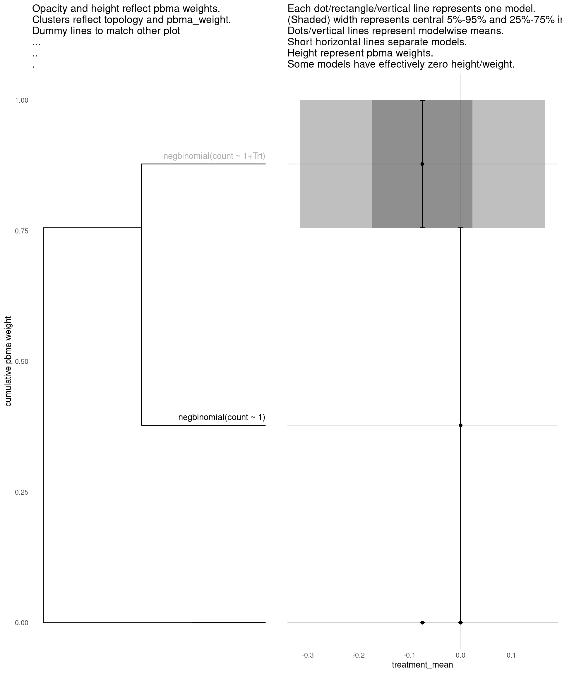
Model with 2 decisions
show_all(
    expand.grid(
        family=names(families),
        Trt=c("","Trt")
    ),
    "treatment_mean"
)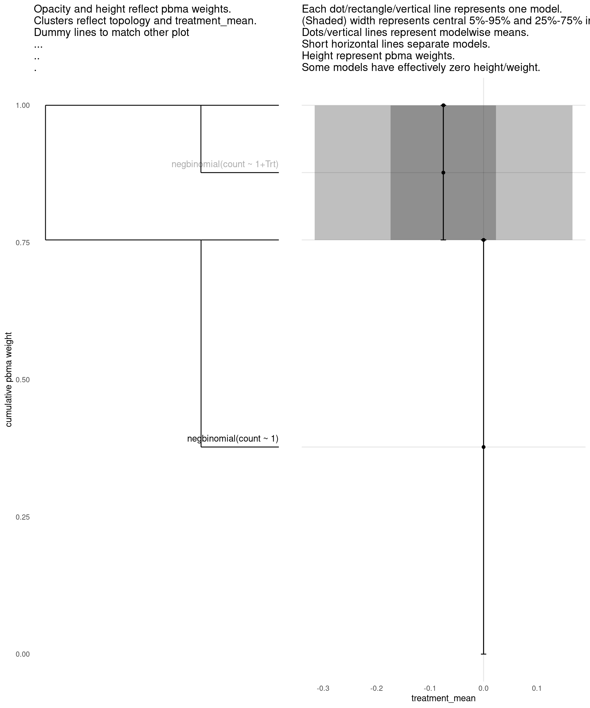
| treatment_mean | pbma_weight | elpd_diff | se_diff | |
|---|---|---|---|---|
| negbinomial(count ~ 1) | 0.00 | 0.75 | 0.00 | 0.00 |
| negbinomial(count ~ 1+Trt) | -0.08 | 0.25 | -1.27 | 0.83 |
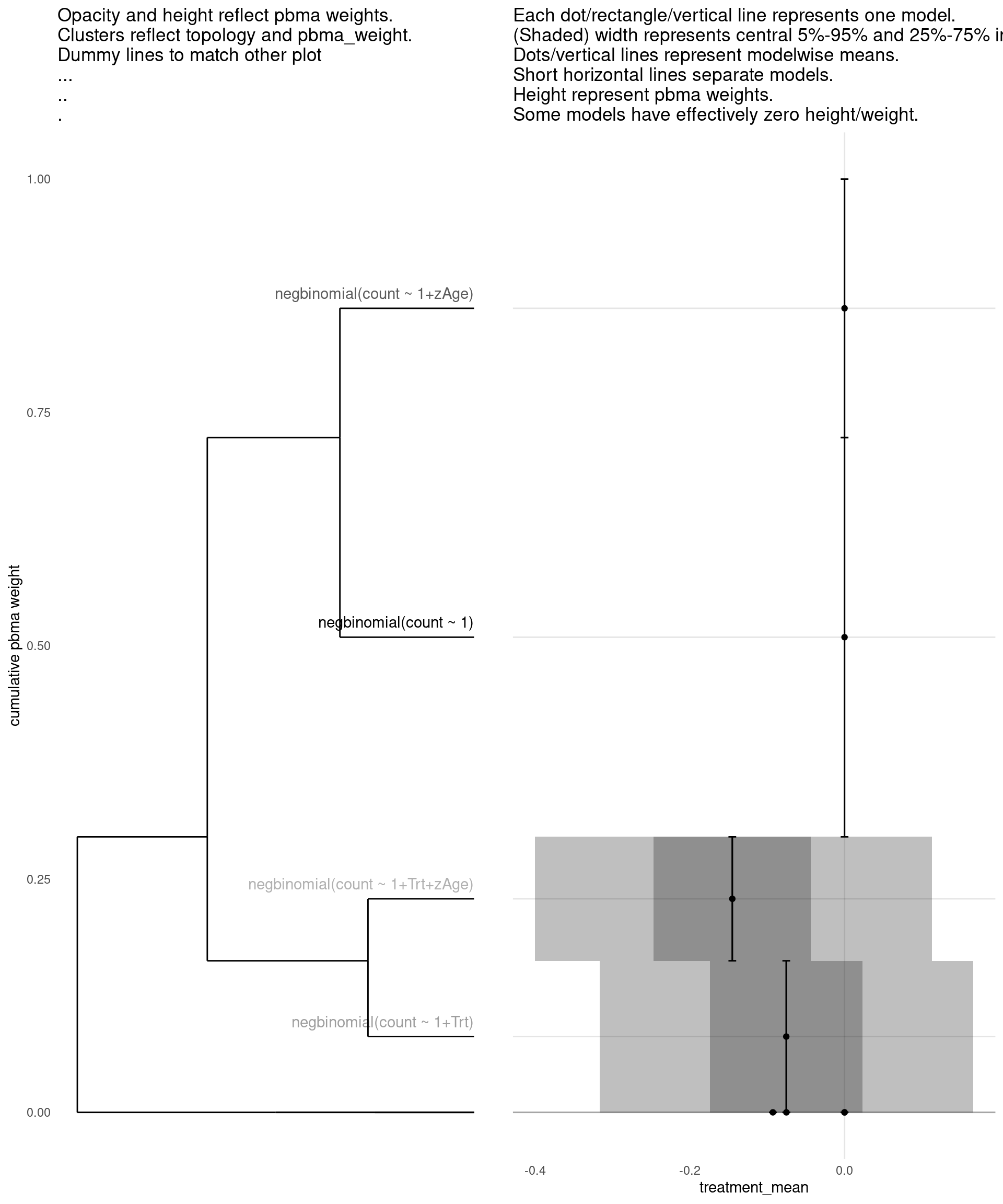
Model with 3 decisions
show_all(
    expand.grid(
        family=names(families),
        Trt=c("","Trt"),
        zAge=c("","zAge")
    ),
    "treatment_mean"
)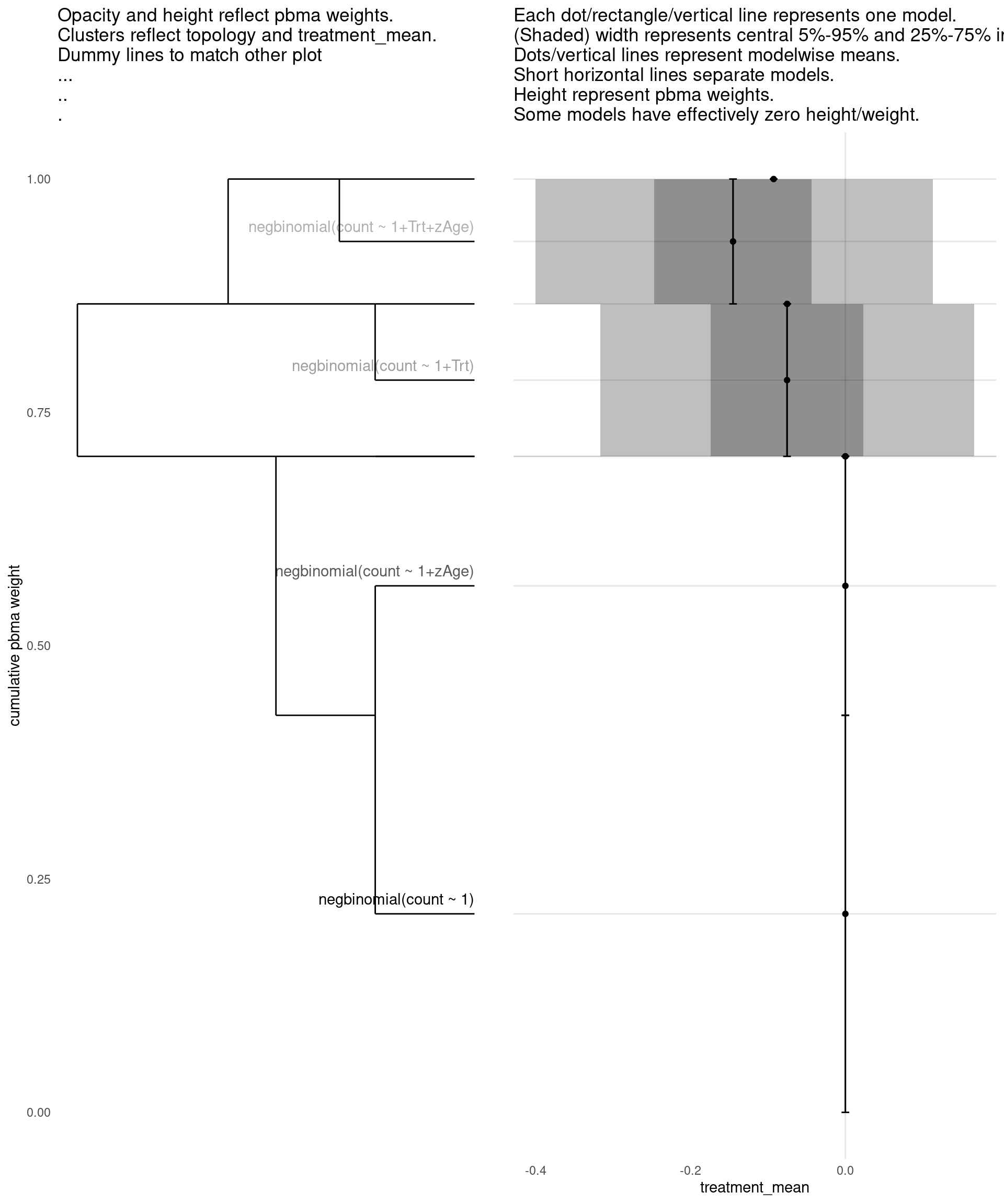
| treatment_mean | pbma_weight | elpd_diff | se_diff | |
|---|---|---|---|---|
| negbinomial(count ~ 1) | 0.00 | 0.42 | 0.00 | 0.00 |
| negbinomial(count ~ 1+zAge) | 0.00 | 0.28 | -0.67 | 1.42 |
| negbinomial(count ~ 1+Trt) | -0.08 | 0.16 | -1.27 | 0.83 |
| negbinomial(count ~ 1+Trt+zAge) | -0.15 | 0.14 | -1.47 | 1.35 |
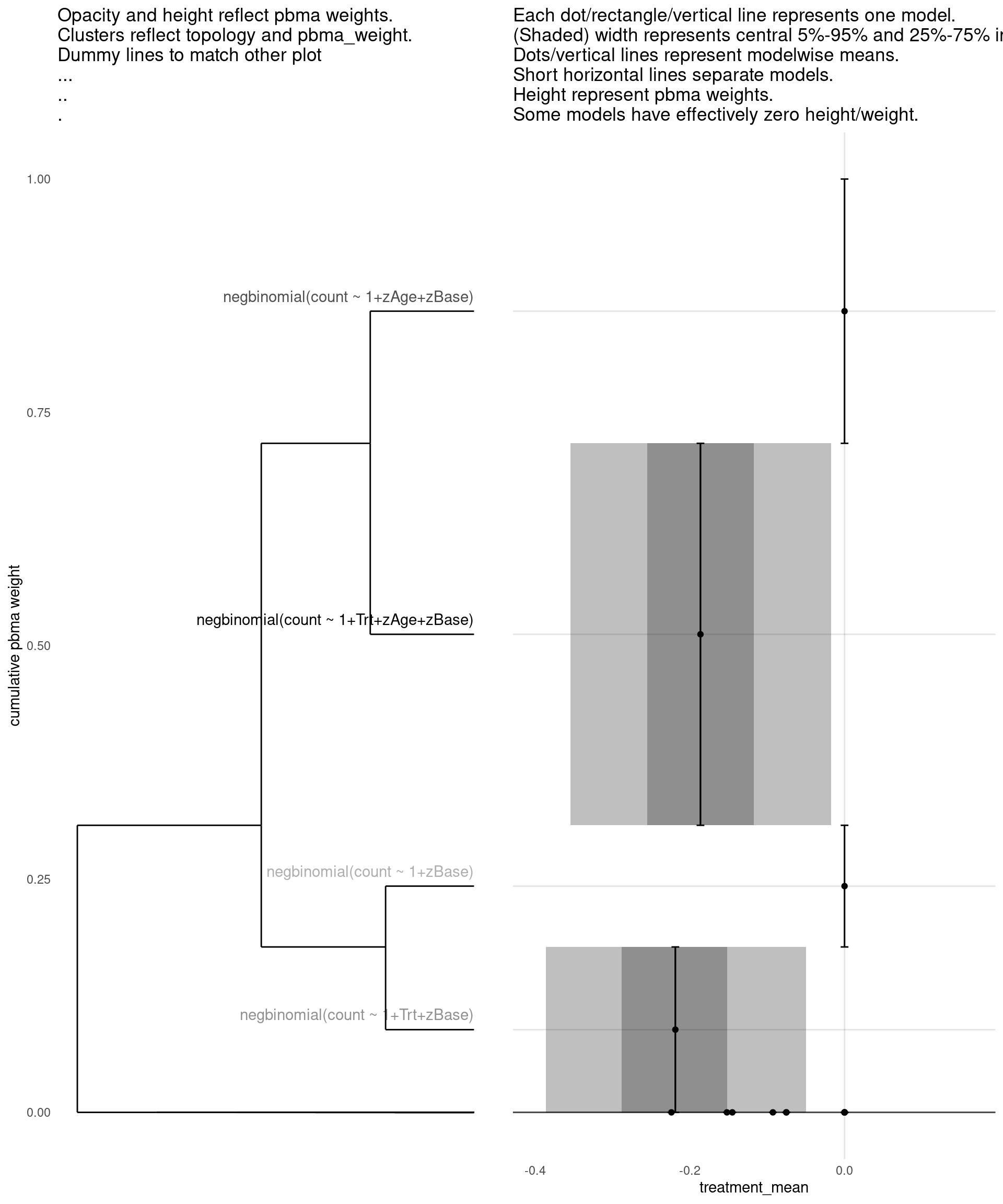
Model with 4 decisions
show_all(
    expand.grid(
        family=names(families),
        Trt=c("","Trt"),
        zAge=c("","zAge"),
        zBase=c("","zBase")
    ),
    "treatment_mean"
)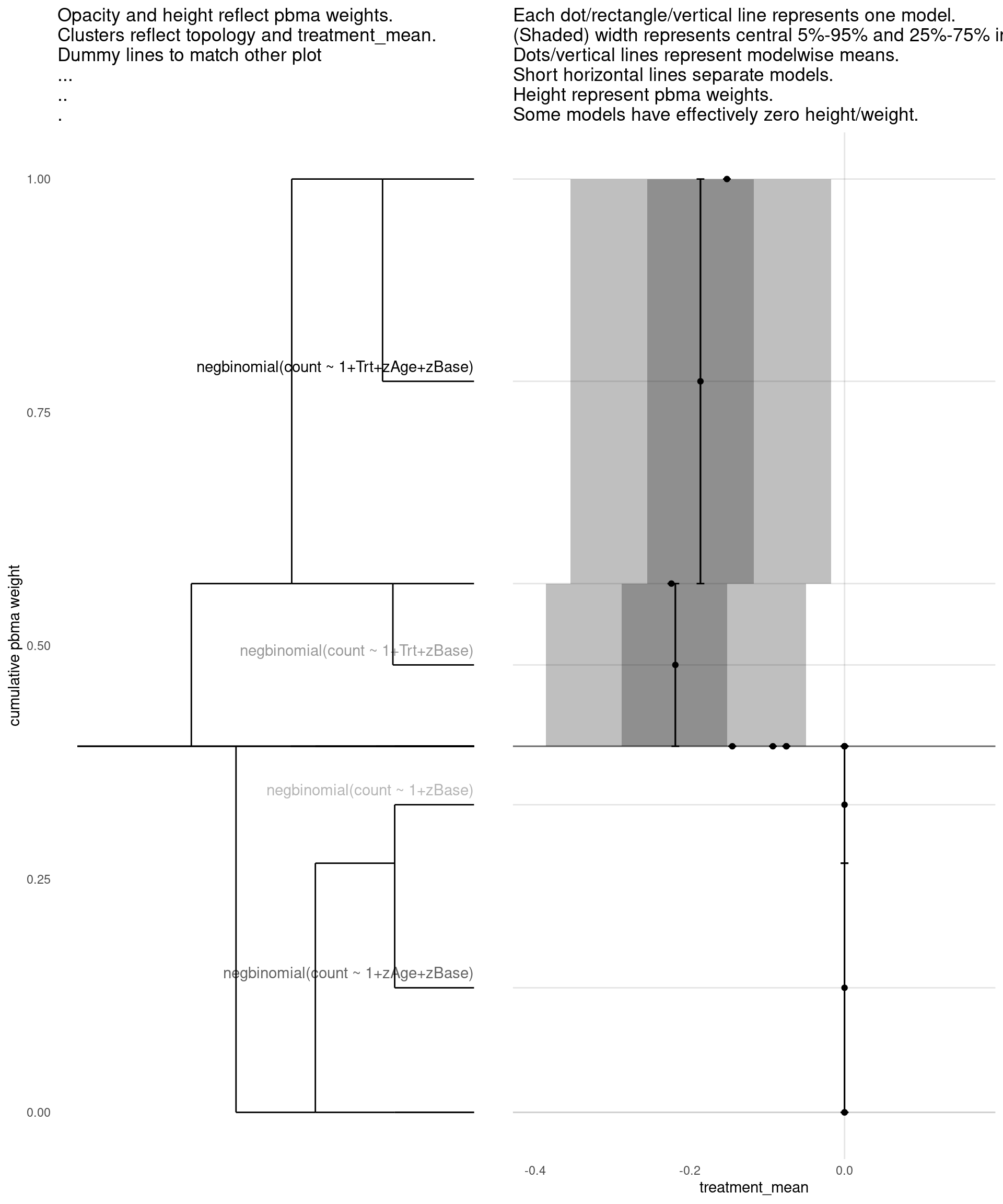
| treatment_mean | pbma_weight | elpd_diff | se_diff | |
|---|---|---|---|---|
| negbinomial(count ~ 1+Trt+zAge+zBase) | -0.19 | 0.41 | 0.00 | 0.00 |
| negbinomial(count ~ 1+zAge+zBase) | 0.00 | 0.29 | -0.65 | 2.03 |
| negbinomial(count ~ 1+Trt+zBase) | -0.22 | 0.18 | -1.40 | 1.90 |
| negbinomial(count ~ 1+zBase) | 0.00 | 0.13 | -2.37 | 3.21 |
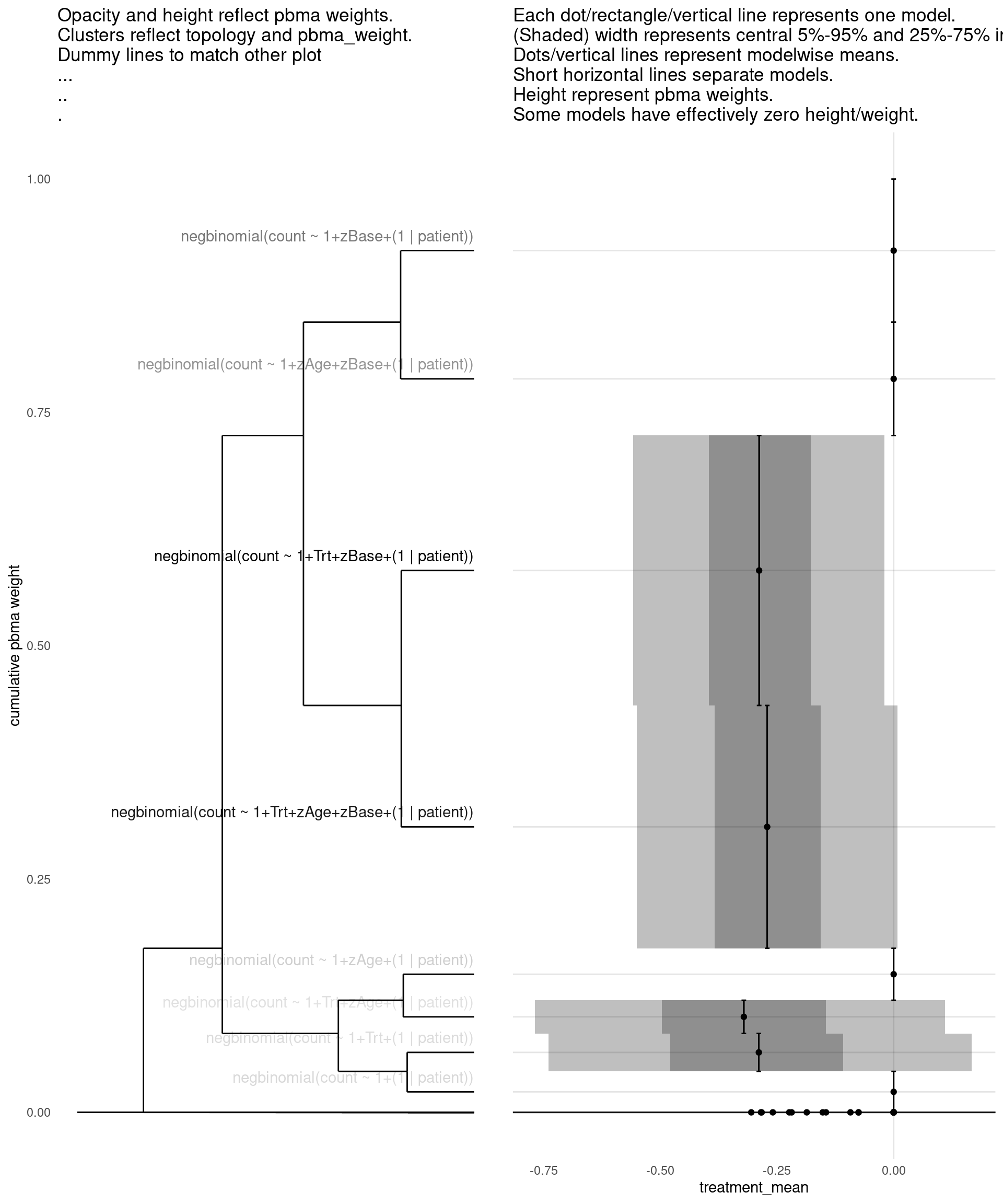
Model with 5 decisions
show_all(
    expand.grid(
        family=names(families),
        Trt=c("","Trt"),
        zAge=c("","zAge"),
        zBase=c("","zBase"),
        patient=c("","(1 | patient)")
    ),
    "treatment_mean"
)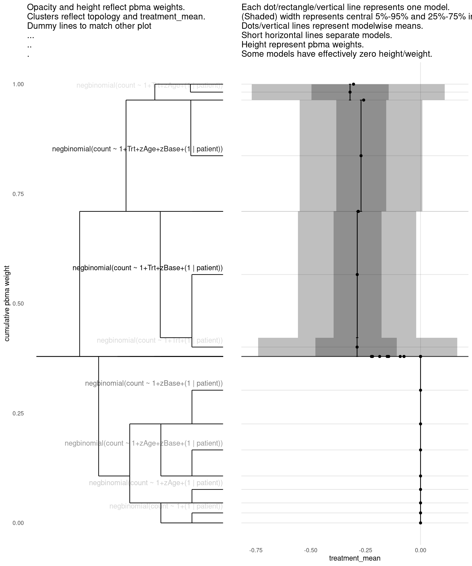
| treatment_mean | pbma_weight | elpd_diff | se_diff | |
|---|---|---|---|---|
| negbinomial(count ~ 1+Trt+zBase+(1 | patient)) | -0.29 | 0.29 | 0.00 | 0.00 |
| negbinomial(count ~ 1+Trt+zAge+zBase+(1 | patient)) | -0.27 | 0.25 | -0.15 | 0.71 |
| negbinomial(count ~ 1+zBase+(1 | patient)) | 0.00 | 0.17 | -0.78 | 1.07 |
| negbinomial(count ~ 1+zAge+zBase+(1 | patient)) | 0.00 | 0.12 | -1.04 | 1.18 |
| negbinomial(count ~ 1+zAge+(1 | patient)) | 0.00 | 0.05 | -3.34 | 3.17 |
| negbinomial(count ~ 1+(1 | patient)) | 0.00 | 0.04 | -3.42 | 3.05 |
| negbinomial(count ~ 1+Trt+(1 | patient)) | -0.29 | 0.04 | -3.66 | 3.12 |
| negbinomial(count ~ 1+Trt+zAge+(1 | patient)) | -0.32 | 0.03 | -3.70 | 3.01 |
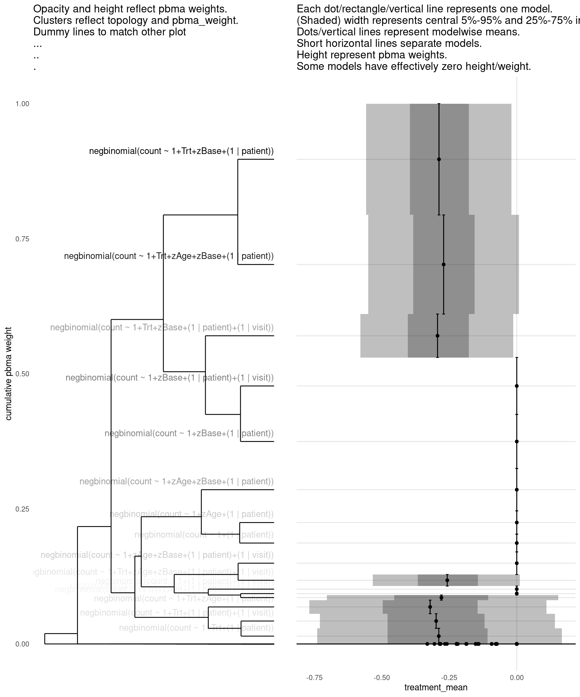
Model with 6 decisions
show_all(
    expand.grid(
        family=names(families),
        Trt=c("","Trt"),
        zAge=c("","zAge"),
        zBase=c("","zBase"),
        patient=c("","(1 | patient)"),
        visit=c("","(1 | visit)")
    ),
    "treatment_mean"
)
| treatment_mean | pbma_weight | elpd_diff | se_diff | |
|---|---|---|---|---|
| negbinomial(count ~ 1+Trt+zBase+(1 | patient)) | -0.29 | 0.21 | 0.00 | 0.00 |
| negbinomial(count ~ 1+Trt+zAge+zBase+(1 | patient)) | -0.27 | 0.19 | -0.15 | 0.71 |
| negbinomial(count ~ 1+zBase+(1 | patient)) | 0.00 | 0.10 | -0.78 | 1.07 |
| negbinomial(count ~ 1+zBase+(1 | patient)+(1 | visit)) | 0.00 | 0.11 | -0.87 | 1.45 |
| negbinomial(count ~ 1+zAge+zBase+(1 | patient)) | 0.00 | 0.08 | -1.04 | 1.18 |
| negbinomial(count ~ 1+Trt+zBase+(1 | patient)+(1 | visit)) | -0.29 | 0.08 | -1.09 | 1.11 |
| negbinomial(count ~ 1+zAge+zBase+(1 | patient)+(1 | visit)) | 0.00 | 0.04 | -1.76 | 1.48 |
| negbinomial(count ~ 1+Trt+zAge+zBase+(1 | patient)+(1 | visit)) | -0.26 | 0.02 | -2.93 | 1.70 |
| negbinomial(count ~ 1+zAge+(1 | patient)) | 0.00 | 0.04 | -3.34 | 3.17 |
| negbinomial(count ~ 1+(1 | patient)) | 0.00 | 0.03 | -3.42 | 3.05 |
| negbinomial(count ~ 1+Trt+(1 | patient)) | -0.29 | 0.03 | -3.66 | 3.12 |
| negbinomial(count ~ 1+Trt+zAge+(1 | patient)) | -0.32 | 0.02 | -3.70 | 3.01 |
| negbinomial(count ~ 1+Trt+(1 | patient)+(1 | visit)) | -0.30 | 0.02 | -3.84 | 3.12 |
| negbinomial(count ~ 1+(1 | patient)+(1 | visit)) | 0.00 | 0.01 | -4.85 | 3.07 |
| negbinomial(count ~ 1+Trt+zAge+(1 | patient)+(1 | visit)) | -0.28 | 0.01 | -4.96 | 3.10 |
| negbinomial(count ~ 1+zAge+(1 | patient)+(1 | visit)) | 0.00 | 0.00 | -5.43 | 3.11 |
| poisson(count ~ 1+zAge+zBase+(1 | patient)+(1 | visit)) | 0.00 | 0.00 | -54.86 | 21.70 |
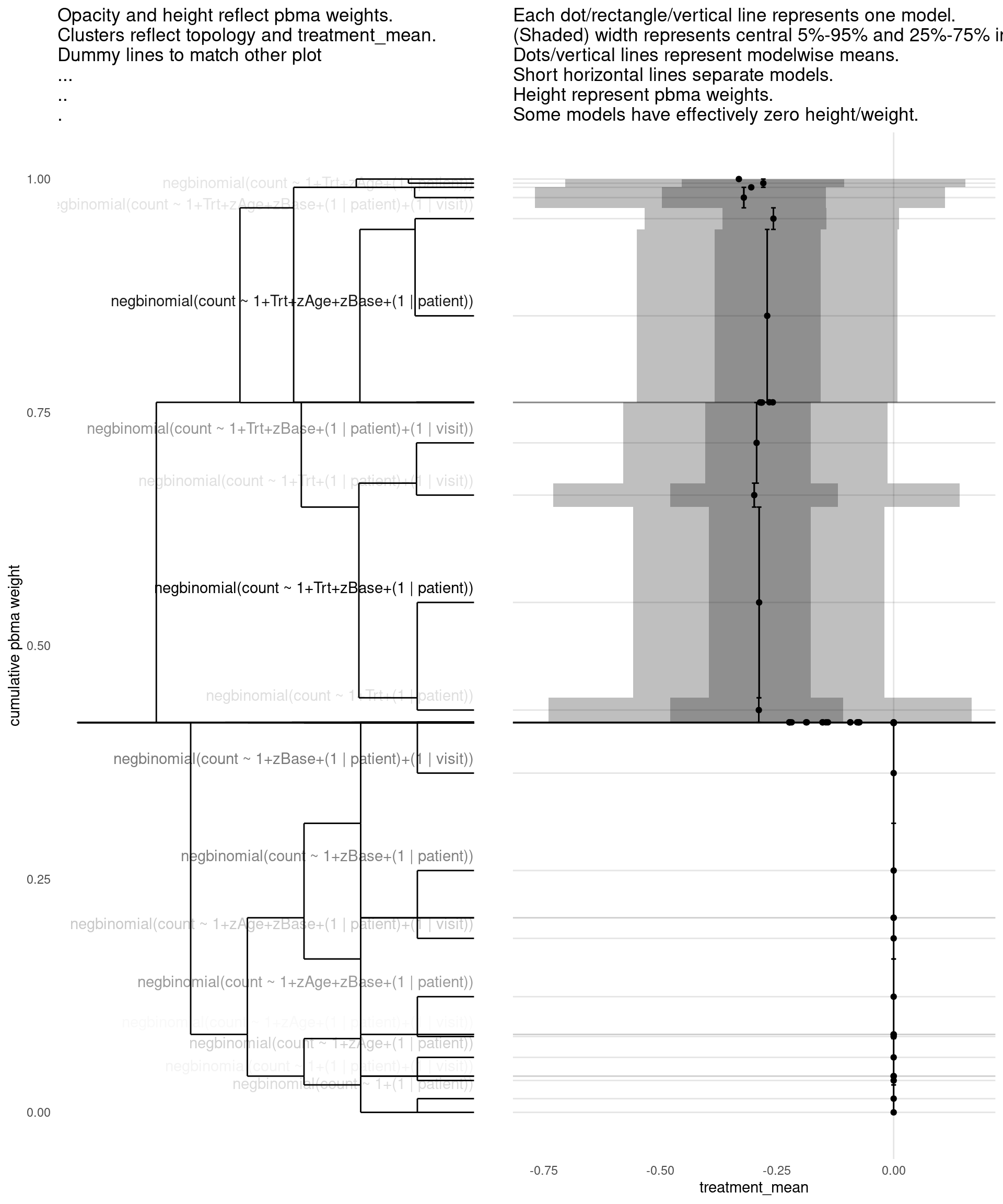
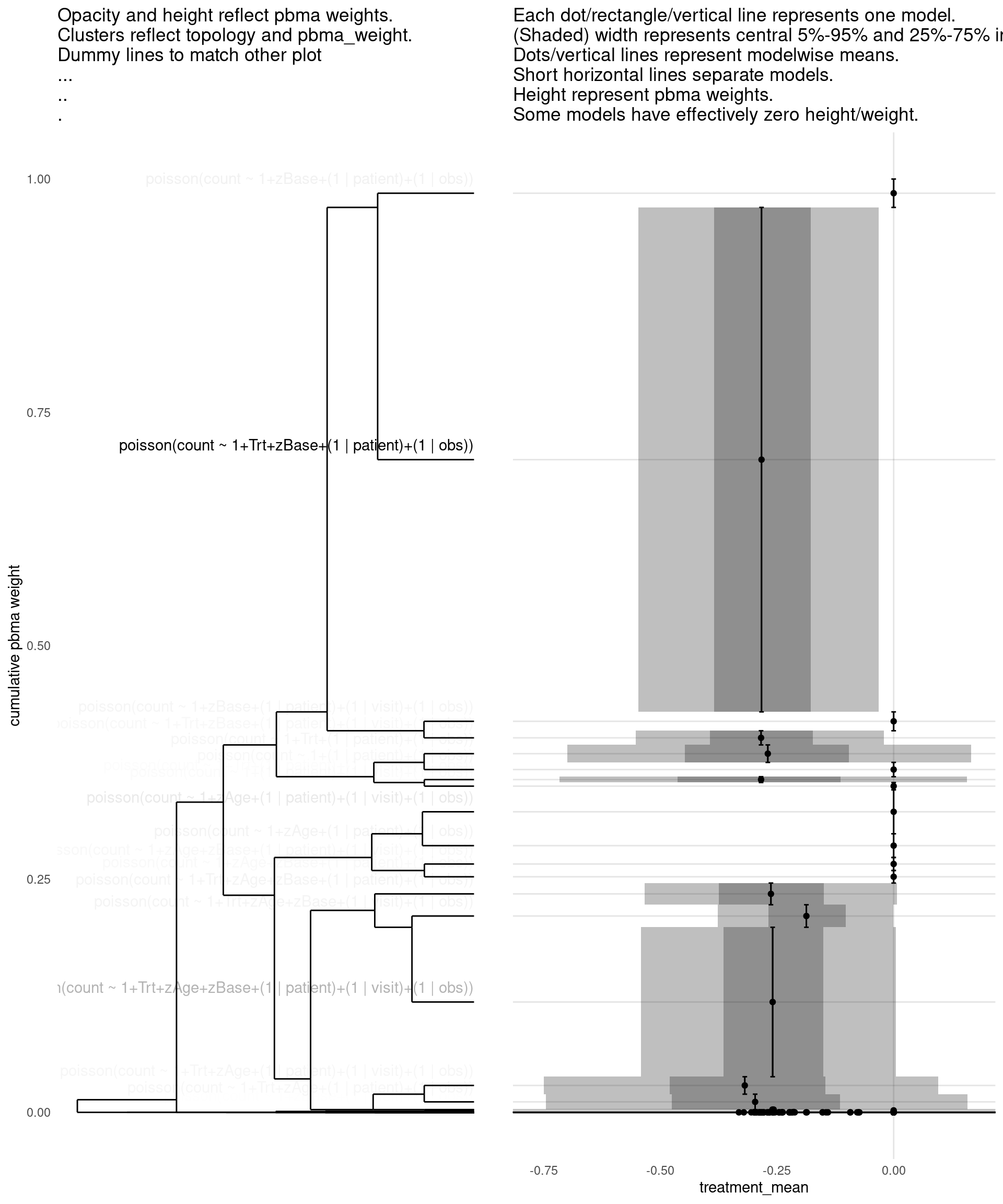
Model with 7 decisions
show_all(
    expand.grid(
        family=names(families),
        Trt=c("","Trt"),
        zAge=c("","zAge"),
        zBase=c("","zBase"),
        patient=c("","(1 | patient)"),
        visit=c("","(1 | visit)"),
        obs=c("","(1 | obs)")
    ),
    "treatment_mean"
)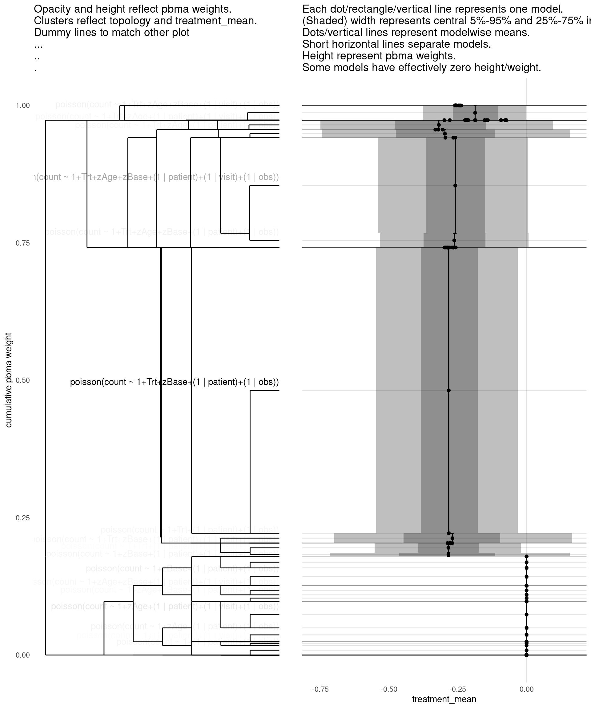
| treatment_mean | pbma_weight | elpd_diff | se_diff | |
|---|---|---|---|---|
| poisson(count ~ 1+Trt+zBase+(1 | patient)+(1 | obs)) | -0.28 | 0.53 | 0.00 | 0.00 |
| poisson(count ~ 1+Trt+zAge+zBase+(1 | patient)+(1 | visit)+(1 | obs)) | -0.26 | 0.17 | -2.01 | 2.24 |
| poisson(count ~ 1+zBase+(1 | patient)+(1 | obs)) | 0.00 | 0.03 | -3.42 | 1.50 |
| poisson(count ~ 1+zBase+(1 | patient)+(1 | visit)+(1 | obs)) | 0.00 | 0.02 | -3.93 | 1.81 |
| poisson(count ~ 1+Trt+zAge+zBase+(1 | patient)+(1 | obs)) | -0.26 | 0.02 | -4.02 | 2.00 |
| poisson(count ~ 1+Trt+zBase+(1 | patient)+(1 | visit)+(1 | obs)) | -0.28 | 0.01 | -4.26 | 1.73 |
| poisson(count ~ 1+zAge+(1 | patient)+(1 | visit)+(1 | obs)) | 0.00 | 0.05 | -4.41 | 3.18 |
| poisson(count ~ 1+zAge+zBase+(1 | patient)+(1 | visit)+(1 | obs)) | 0.00 | 0.02 | -4.44 | 1.92 |
| poisson(count ~ 1+zAge+zBase+(1 | patient)+(1 | obs)) | 0.00 | 0.01 | -4.97 | 2.15 |
| poisson(count ~ 1+zAge+(1 | patient)+(1 | obs)) | 0.00 | 0.02 | -5.34 | 3.33 |
| poisson(count ~ 1+Trt+(1 | patient)+(1 | obs)) | -0.27 | 0.02 | -5.35 | 3.09 |
| poisson(count ~ 1+(1 | patient)+(1 | obs)) | 0.00 | 0.02 | -5.54 | 3.16 |
| poisson(count ~ 1+Trt+zAge+(1 | patient)+(1 | obs)) | -0.30 | 0.02 | -5.78 | 3.39 |
| poisson(count ~ 1+Trt+zAge+(1 | patient)+(1 | visit)+(1 | obs)) | -0.32 | 0.02 | -5.99 | 3.63 |
| poisson(count ~ 1+Trt+(1 | patient)+(1 | visit)+(1 | obs)) | -0.28 | 0.01 | -6.33 | 3.00 |
| poisson(count ~ 1+(1 | patient)+(1 | visit)+(1 | obs)) | 0.00 | 0.01 | -6.77 | 3.55 |
| negbinomial(count ~ 1+Trt+zBase+(1 | patient)+(1 | obs)) | -0.27 | 0.00 | -14.60 | 3.55 |
| negbinomial(count ~ 1+zAge+zBase+(1 | patient)+(1 | visit)+(1 | obs)) | 0.00 | 0.00 | -16.07 | 4.70 |
| poisson(count ~ 1+Trt+zAge+zBase+(1 | visit)+(1 | obs)) | -0.19 | 0.03 | -16.36 | 8.05 |
| negbinomial(count ~ 1+zAge+zBase+(1 | patient)+(1 | obs)) | 0.00 | 0.00 | -16.52 | 4.13 |
| poisson(count ~ 1+Trt+zAge+zBase+(1 | obs)) | -0.21 | 0.00 | -21.03 | 7.71 |
| poisson(count ~ 1+zBase+(1 | visit)+(1 | obs)) | 0.00 | 0.00 | -22.50 | 7.96 |
| poisson(count ~ 1+Trt+zBase+(1 | visit)+(1 | obs)) | -0.24 | 0.00 | -22.53 | 7.88 |
| poisson(count ~ 1+zAge+zBase+(1 | obs)) | 0.00 | 0.00 | -23.05 | 8.08 |
| poisson(count ~ 1+zAge+zBase+(1 | visit)+(1 | obs)) | 0.00 | 0.00 | -23.59 | 8.31 |
| poisson(count ~ 1+Trt+zBase+(1 | obs)) | -0.24 | 0.00 | -24.05 | 7.79 |
| poisson(count ~ 1+zBase+(1 | obs)) | 0.00 | 0.00 | -26.52 | 8.02 |
Visualizations, clustered by pbma_weight
Model with 2 decisions
show_all(
    expand.grid(
        family=names(families),
        Trt=c("","Trt")
    ),
    "pbma_weight"
)
| treatment_mean | pbma_weight | elpd_diff | se_diff | |
|---|---|---|---|---|
| negbinomial(count ~ 1) | 0.00 | 0.75 | 0.00 | 0.00 |
| negbinomial(count ~ 1+Trt) | -0.08 | 0.25 | -1.27 | 0.83 |
Model with 3 decisions
show_all(
    expand.grid(
        family=names(families),
        Trt=c("","Trt"),
        zAge=c("","zAge")
    ),
    "pbma_weight"
)
| treatment_mean | pbma_weight | elpd_diff | se_diff | |
|---|---|---|---|---|
| negbinomial(count ~ 1) | 0.00 | 0.43 | 0.00 | 0.00 |
| negbinomial(count ~ 1+zAge) | 0.00 | 0.28 | -0.67 | 1.42 |
| negbinomial(count ~ 1+Trt) | -0.08 | 0.16 | -1.27 | 0.83 |
| negbinomial(count ~ 1+Trt+zAge) | -0.15 | 0.13 | -1.47 | 1.35 |
Model with 4 decisions
show_all(
    expand.grid(
        family=names(families),
        Trt=c("","Trt"),
        zAge=c("","zAge"),
        zBase=c("","zBase")
    ),
    "pbma_weight"
)
| treatment_mean | pbma_weight | elpd_diff | se_diff | |
|---|---|---|---|---|
| negbinomial(count ~ 1+Trt+zAge+zBase) | -0.19 | 0.42 | 0.00 | 0.00 |
| negbinomial(count ~ 1+zAge+zBase) | 0.00 | 0.28 | -0.65 | 2.03 |
| negbinomial(count ~ 1+Trt+zBase) | -0.22 | 0.18 | -1.40 | 1.90 |
| negbinomial(count ~ 1+zBase) | 0.00 | 0.12 | -2.37 | 3.21 |
Model with 5 decisions
show_all(
    expand.grid(
        family=names(families),
        Trt=c("","Trt"),
        zAge=c("","zAge"),
        zBase=c("","zBase"),
        patient=c("","(1 | patient)")
    ),
    "pbma_weight"
)
| treatment_mean | pbma_weight | elpd_diff | se_diff | |
|---|---|---|---|---|
| negbinomial(count ~ 1+Trt+zBase+(1 | patient)) | -0.29 | 0.28 | 0.00 | 0.00 |
| negbinomial(count ~ 1+Trt+zAge+zBase+(1 | patient)) | -0.27 | 0.26 | -0.15 | 0.71 |
| negbinomial(count ~ 1+zBase+(1 | patient)) | 0.00 | 0.15 | -0.78 | 1.07 |
| negbinomial(count ~ 1+zAge+zBase+(1 | patient)) | 0.00 | 0.12 | -1.04 | 1.18 |
| negbinomial(count ~ 1+zAge+(1 | patient)) | 0.00 | 0.06 | -3.34 | 3.17 |
| negbinomial(count ~ 1+(1 | patient)) | 0.00 | 0.05 | -3.42 | 3.05 |
| negbinomial(count ~ 1+Trt+(1 | patient)) | -0.29 | 0.04 | -3.66 | 3.12 |
| negbinomial(count ~ 1+Trt+zAge+(1 | patient)) | -0.32 | 0.04 | -3.70 | 3.01 |
| poisson(count ~ 1+Trt+zBase+(1 | patient)) | -0.28 | 0.00 | -54.81 | 22.23 |
| poisson(count ~ 1+zBase+(1 | patient)) | 0.00 | 0.00 | -54.91 | 22.05 |
Model with 6 decisions
show_all(
    expand.grid(
        family=names(families),
        Trt=c("","Trt"),
        zAge=c("","zAge"),
        zBase=c("","zBase"),
        patient=c("","(1 | patient)"),
        visit=c("","(1 | visit)")
    ),
    "pbma_weight"
)
| treatment_mean | pbma_weight | elpd_diff | se_diff | |
|---|---|---|---|---|
| negbinomial(count ~ 1+Trt+zBase+(1 | patient)) | -0.29 | 0.19 | 0.00 | 0.00 |
| negbinomial(count ~ 1+Trt+zAge+zBase+(1 | patient)) | -0.27 | 0.19 | -0.15 | 0.71 |
| negbinomial(count ~ 1+zBase+(1 | patient)) | 0.00 | 0.10 | -0.78 | 1.07 |
| negbinomial(count ~ 1+zBase+(1 | patient)+(1 | visit)) | 0.00 | 0.11 | -0.87 | 1.45 |
| negbinomial(count ~ 1+zAge+zBase+(1 | patient)) | 0.00 | 0.08 | -1.04 | 1.18 |
| negbinomial(count ~ 1+Trt+zBase+(1 | patient)+(1 | visit)) | -0.29 | 0.08 | -1.09 | 1.11 |
| negbinomial(count ~ 1+zAge+zBase+(1 | patient)+(1 | visit)) | 0.00 | 0.05 | -1.76 | 1.48 |
| negbinomial(count ~ 1+Trt+zAge+zBase+(1 | patient)+(1 | visit)) | -0.26 | 0.02 | -2.93 | 1.70 |
| negbinomial(count ~ 1+zAge+(1 | patient)) | 0.00 | 0.04 | -3.34 | 3.17 |
| negbinomial(count ~ 1+(1 | patient)) | 0.00 | 0.03 | -3.42 | 3.05 |
| negbinomial(count ~ 1+Trt+(1 | patient)) | -0.29 | 0.03 | -3.66 | 3.12 |
| negbinomial(count ~ 1+Trt+zAge+(1 | patient)) | -0.32 | 0.02 | -3.70 | 3.01 |
| negbinomial(count ~ 1+Trt+(1 | patient)+(1 | visit)) | -0.30 | 0.03 | -3.84 | 3.12 |
| negbinomial(count ~ 1+(1 | patient)+(1 | visit)) | 0.00 | 0.01 | -4.85 | 3.07 |
| negbinomial(count ~ 1+Trt+zAge+(1 | patient)+(1 | visit)) | -0.28 | 0.01 | -4.96 | 3.10 |
| negbinomial(count ~ 1+zAge+(1 | patient)+(1 | visit)) | 0.00 | 0.01 | -5.43 | 3.11 |
Model with 7 decisions
show_all(
    expand.grid(
        family=names(families),
        Trt=c("","Trt"),
        zAge=c("","zAge"),
        zBase=c("","zBase"),
        patient=c("","(1 | patient)"),
        visit=c("","(1 | visit)"),
        obs=c("","(1 | obs)")
    ),
    "pbma_weight"
)
| treatment_mean | pbma_weight | elpd_diff | se_diff | |
|---|---|---|---|---|
| poisson(count ~ 1+Trt+zBase+(1 | patient)+(1 | obs)) | -0.28 | 0.54 | 0.00 | 0.00 |
| poisson(count ~ 1+Trt+zAge+zBase+(1 | patient)+(1 | visit)+(1 | obs)) | -0.26 | 0.16 | -2.01 | 2.24 |
| poisson(count ~ 1+zBase+(1 | patient)+(1 | obs)) | 0.00 | 0.03 | -3.42 | 1.50 |
| poisson(count ~ 1+zBase+(1 | patient)+(1 | visit)+(1 | obs)) | 0.00 | 0.02 | -3.93 | 1.81 |
| poisson(count ~ 1+Trt+zAge+zBase+(1 | patient)+(1 | obs)) | -0.26 | 0.02 | -4.02 | 2.00 |
| poisson(count ~ 1+Trt+zBase+(1 | patient)+(1 | visit)+(1 | obs)) | -0.28 | 0.02 | -4.26 | 1.73 |
| poisson(count ~ 1+zAge+(1 | patient)+(1 | visit)+(1 | obs)) | 0.00 | 0.04 | -4.41 | 3.18 |
| poisson(count ~ 1+zAge+zBase+(1 | patient)+(1 | visit)+(1 | obs)) | 0.00 | 0.02 | -4.44 | 1.92 |
| poisson(count ~ 1+zAge+zBase+(1 | patient)+(1 | obs)) | 0.00 | 0.01 | -4.97 | 2.15 |
| poisson(count ~ 1+zAge+(1 | patient)+(1 | obs)) | 0.00 | 0.02 | -5.34 | 3.33 |
| poisson(count ~ 1+Trt+(1 | patient)+(1 | obs)) | -0.27 | 0.02 | -5.35 | 3.09 |
| poisson(count ~ 1+(1 | patient)+(1 | obs)) | 0.00 | 0.02 | -5.54 | 3.16 |
| poisson(count ~ 1+Trt+zAge+(1 | patient)+(1 | obs)) | -0.30 | 0.01 | -5.78 | 3.39 |
| poisson(count ~ 1+Trt+zAge+(1 | patient)+(1 | visit)+(1 | obs)) | -0.32 | 0.02 | -5.99 | 3.63 |
| poisson(count ~ 1+Trt+(1 | patient)+(1 | visit)+(1 | obs)) | -0.28 | 0.01 | -6.33 | 3.00 |
| poisson(count ~ 1+(1 | patient)+(1 | visit)+(1 | obs)) | 0.00 | 0.01 | -6.77 | 3.55 |
| negbinomial(count ~ 1+Trt+zBase+(1 | patient)+(1 | obs)) | -0.27 | 0.00 | -14.60 | 3.55 |
| negbinomial(count ~ 1+zAge+zBase+(1 | patient)+(1 | visit)+(1 | obs)) | 0.00 | 0.00 | -16.07 | 4.70 |
| poisson(count ~ 1+Trt+zAge+zBase+(1 | visit)+(1 | obs)) | -0.19 | 0.03 | -16.36 | 8.05 |
| negbinomial(count ~ 1+zAge+zBase+(1 | patient)+(1 | obs)) | 0.00 | 0.00 | -16.52 | 4.13 |
| poisson(count ~ 1+Trt+zAge+zBase+(1 | obs)) | -0.21 | 0.00 | -21.03 | 7.71 |
| poisson(count ~ 1+zBase+(1 | visit)+(1 | obs)) | 0.00 | 0.00 | -22.50 | 7.96 |
| poisson(count ~ 1+Trt+zBase+(1 | visit)+(1 | obs)) | -0.24 | 0.00 | -22.53 | 7.88 |
| poisson(count ~ 1+zAge+zBase+(1 | obs)) | 0.00 | 0.00 | -23.05 | 8.08 |
| poisson(count ~ 1+zAge+zBase+(1 | visit)+(1 | obs)) | 0.00 | 0.00 | -23.59 | 8.31 |
| poisson(count ~ 1+Trt+zBase+(1 | obs)) | -0.24 | 0.00 | -24.05 | 7.79 |
| poisson(count ~ 1+zBase+(1 | obs)) | 0.00 | 0.00 | -26.52 | 8.02 |
| poisson(count ~ 1+(1 | obs)) | 0.00 | 0.00 | -37.58 | 9.33 |