Adaptive HSGP centering
The difficult geometry of a Gaussian process is not necessarily resolved by choosing one centered or noncentered parameterization for every coefficient. Low and high HSGP frequencies can need different coordinates. This case study follows Generable's motorcycle example: fit the noncentered model, inspect its geometry, choose one centering per basis weight, and fit the reparameterized model from scratch.
The source workflow has a noncentered pilot and a selected-partial refit. This extension compares both adaptation losses, post-hoc and online, alongside fixed CP and NCP controls. Centered geometry remains the visual reference.
The model
All 133 MASS::mcycle observations are used. A zero-mean squared-exponential HSGP models the conditional mean, and another models the log conditional standard deviation:
mu(t)  = HSGP_mu(t)
eta(t) = HSGP_sigma(t)
y(t) ~ Normal(mu(t), exp(eta(t)))
Acceleration is divided by its sample standard deviation. Time is mapped to [-1,1]. Each GP has 20 sine basis functions on [-1.5,1.5], with the source's 1/sqrt(1.5) normalization. There is no additional population intercept.
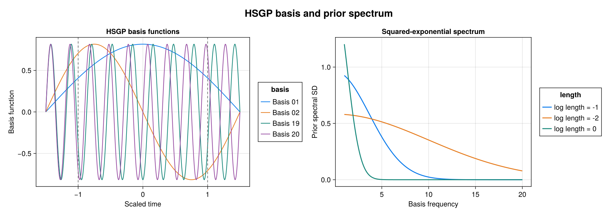
The left panel shows frequencies 1, 2, 19 and 20; the dotted vertical lines mark the observed domain. The right panel shows how increasing the length scale suppresses the high-frequency weights.
Hyperpriors and source equivalence
The source assigns independent Normal(0,4) priors to the log length scale and log marginal standard deviation of each GP. BRM expresses these as LogNormal(0,4) on the four positive parameters. The change of variables is part of that equivalence:
logpdf(LogNormal(0,4), exp(q)) + q = logpdf(Normal(0,4), q)The +q is the unconstraining Jacobian. Each positive parameter has support (0, Inf), with no additional length-scale floor.
research/adaptive_centering/audit_source.jl compiles the immutable original Stan program and compares it with the actual BRM-generated Stan model. Its 26 noncentered-model checks cover the coordinate mapping, normalized target including the Jacobian, and all 44 gradient components. Across six tested points the largest absolute density and gradient differences were 5.7e-14 and 4.3e-14. The companion audit_partial_source.jl checks the fresh partial model against the original adaptive Stan program at 16 saved posterior positions. All 51 checks pass; the largest density and gradient differences are 9.95e-14 and 5.59e-12. These are comparisons of the actual generated targets, including the source hyperpriors, not just algebraic prior identities.
One BRM formula and its generated backends
This executable example reads the full dataset and uses the same 20-frequency model as the sampling runs. The tabs expose its generated backends. All fits on this page use StanBlocks/BridgeStan; the Turing tab shows generated code.
The full motorcycle modelusing Statistics
function adaptive_motorcycle_model()
csv = joinpath(dirname(pathof(BayesianRegressionModels)), "..",
"research", "adaptive_centering", "mcycle.csv")
rows = split.(readlines(csv)[2:end], ',')
times = parse.(Float64, getindex.(rows, 2))
accel = parse.(Float64, getindex.(rows, 3))
xmin, xmax = extrema(times)
x = @. -1 + 2 * (times - xmin) / (xmax - xmin)
y = accel ./ std(accel)
(@brm begin
length_scale(mu, hsgp(x)) ~ LogNormal(0, 4)
sd(mu, hsgp(x)) ~ LogNormal(0, 4)
length_scale(sigma, hsgp(x)) ~ LogNormal(0, 4)
sd(sigma, hsgp(x)) ~ LogNormal(0, 4)
mu ~ hsgp(x; k=20, domain=(-1.5, 1.5))
log(sigma) ~ hsgp(x; k=20, domain=(-1.5, 1.5))
y ~ Normal(mu, sigma)
end)((; x, y))
endBRMI:
effect(term_length_scale, hsgp(x), mu) ~ LogNormal(0, 4)
effect(term_sd, hsgp(x), mu) ~ LogNormal(0, 4)
effect(term_length_scale, hsgp(x), sigma) ~ LogNormal(0, 4)
effect(term_sd, hsgp(x), sigma) ~ LogNormal(0, 4)
x: data (eltype=Float64, n=133)
mu ~ hsgp(x; k=20, domain=(-1.5, 1.5))
log(sigma) ~ hsgp(x; k=20, domain=(-1.5, 1.5))
y ~ Normal(mu, sigma)SBBRMI with data keys = [:PHI_hsgp_log_sigma_x, :PHI_hsgp_x, :omega2_hsgp_log_sigma_x, :omega2_hsgp_x, :rho_lower_hsgp_log_sigma_x, :rho_lower_hsgp_x, :x, :y]
configured submodels:
_sb_hsgp_configured_1 = Base.merge(BayesianRegressionModels._sb_hsgp, quote
rho_iso ~ lognormal(0.0, 4.0; lower = 0.0)
sigma ~ lognormal(0.0, 4.0; lower = 0.0)
end)
emitted @slic body:
begin
hsgp_x ~ _sb_hsgp_configured_1(; PHI = PHI_hsgp_x, omega2 = omega2_hsgp_x, rho_lower = rho_lower_hsgp_x)
mu = hsgp_x
hsgp_log_sigma_x ~ _sb_hsgp_configured_1(; PHI = PHI_hsgp_log_sigma_x, omega2 = omega2_hsgp_log_sigma_x, rho_lower = rho_lower_hsgp_log_sigma_x)
log_sigma = hsgp_log_sigma_x
sigma = exp(log_sigma)
y ~ normal(mu, sigma)
endfunctions {
vector brm_hsgp_sqrt_spd(
matrix omega2,
real sigma,
vector rho
) {
int m = dims(omega2)[1];
int d = dims(omega2)[2];
if (dims(rho)[1] != d) reject("brm_hsgp_sqrt_spd: dim mismatch — `rho` dim 1 (= ", dims(rho)[1], ") does not match `d` (= ", d, "), inferred from `omega2` dim 2. `d` sizes: `omega2` dim 2 (= ", dims(omega2)[2], "), `rho` dim 1 (= ", dims(rho)[1], ").");
vector[m] rv;
real scale = sigma;
for(axis in 1:d) {
scale *= sqrt((rho[axis] * 2.5066282746310002));
}
for(b in 1:m) {
real exponent = 0.0;
for(axis in 1:d) {
exponent += (rho[axis] * rho[axis] * omega2[b, axis]);
}
rv[b] = (scale * exp((-0.25 * exponent)));
}
return rv;
}
vector normal_lpdfs(
vector obs,
vector loc,
vector scale
) {
return jbroadcasted_normal_lpdfs(obs, loc, scale);
}
vector jbroadcasted_normal_lpdfs(
vector x1,
vector x2,
vector x3
) {
int n = dims(x1)[1];
vector[n] rv;
for(i in 1:n) {
rv[i] = normal_lpdfs(broadcasted_getindex(x1, i), broadcasted_getindex(x2, i), broadcasted_getindex(x3, i));
}
return rv;
}
real normal_lpdfs(
real args1,
real args2,
real args3
) {
return normal_lpdf(args1 | args2, args3);
}
real broadcasted_getindex(vector x, int i) {
return x[i];
}
vector normal_vector_rng(
int anontok__1,
vector a,
vector b
) {
int n = anontok__1;
if((n == 0)) {
vector[n] rv;
return rv;
} else {
return to_vector(normal_rng(a, b));
}
}
}
data {
int omega2_hsgp_x_m;
int omega2_hsgp_x_n;
matrix[omega2_hsgp_x_m, omega2_hsgp_x_n] omega2_hsgp_x;
int PHI_hsgp_x_m;
int PHI_hsgp_x_n;
matrix[PHI_hsgp_x_m, PHI_hsgp_x_n] PHI_hsgp_x;
int omega2_hsgp_log_sigma_x_m;
int omega2_hsgp_log_sigma_x_n;
matrix[omega2_hsgp_log_sigma_x_m, omega2_hsgp_log_sigma_x_n] omega2_hsgp_log_sigma_x;
int PHI_hsgp_log_sigma_x_m;
int PHI_hsgp_log_sigma_x_n;
matrix[PHI_hsgp_log_sigma_x_m, PHI_hsgp_log_sigma_x_n] PHI_hsgp_log_sigma_x;
int y_n;
vector[y_n] y;
}
transformed data {
int hsgp_x_n_basis = omega2_hsgp_x_m;
int hsgp_x_n_axes = omega2_hsgp_x_n;
int hsgp_log_sigma_x_n_basis = omega2_hsgp_log_sigma_x_m;
int hsgp_log_sigma_x_n_axes = omega2_hsgp_log_sigma_x_n;
}
parameters {
real<lower=0.0> hsgp_x_rho_iso;
real<lower=0.0> hsgp_x_sigma;
vector[hsgp_x_n_basis] hsgp_x_beta_raw;
real<lower=0.0> hsgp_log_sigma_x_rho_iso;
real<lower=0.0> hsgp_log_sigma_x_sigma;
vector[hsgp_log_sigma_x_n_basis] hsgp_log_sigma_x_beta_raw;
}
transformed parameters {
vector[hsgp_x_n_axes] hsgp_x_rho = rep_vector(hsgp_x_rho_iso, hsgp_x_n_axes);
vector[omega2_hsgp_x_m] hsgp_x_sqrt_spd = brm_hsgp_sqrt_spd(omega2_hsgp_x, hsgp_x_sigma, hsgp_x_rho);
vector[PHI_hsgp_x_m] hsgp_x = (PHI_hsgp_x * (hsgp_x_sqrt_spd .* hsgp_x_beta_raw));
vector[PHI_hsgp_x_m] mu = hsgp_x;
vector[hsgp_log_sigma_x_n_axes] hsgp_log_sigma_x_rho = rep_vector(hsgp_log_sigma_x_rho_iso, hsgp_log_sigma_x_n_axes);
vector[omega2_hsgp_log_sigma_x_m] hsgp_log_sigma_x_sqrt_spd = brm_hsgp_sqrt_spd(omega2_hsgp_log_sigma_x, hsgp_log_sigma_x_sigma, hsgp_log_sigma_x_rho);
vector[PHI_hsgp_log_sigma_x_m] hsgp_log_sigma_x = (PHI_hsgp_log_sigma_x * (hsgp_log_sigma_x_sqrt_spd .* hsgp_log_sigma_x_beta_raw));
vector[PHI_hsgp_log_sigma_x_m] log_sigma = hsgp_log_sigma_x;
vector[PHI_hsgp_log_sigma_x_m] sigma = exp(log_sigma);
}
model {
hsgp_x_rho_iso ~ lognormal(0.0, 4.0);
hsgp_x_sigma ~ lognormal(0.0, 4.0);
hsgp_x_beta_raw ~ std_normal();
hsgp_log_sigma_x_rho_iso ~ lognormal(0.0, 4.0);
hsgp_log_sigma_x_sigma ~ lognormal(0.0, 4.0);
hsgp_log_sigma_x_beta_raw ~ std_normal();
y ~ normal(mu, sigma);
}
generated quantities {
vector[y_n] y_likelihood = normal_lpdfs(y, mu, sigma);
vector[y_n] y_gen = normal_vector_rng(y_n, mu, sigma);
}#= line 0 =# Turing.@model(function brm_model(y, terms_mu_1, x, terms_sigma_1)
term_mu_1 ~ DynamicPPL.to_submodel(BayesianRegressionModelsTuringExt._brm_turing_hsgp_ncp_model(terms_mu_1, Base.length(y), NamedTuple{$(QuoteNode((:rho, :sigma)))}((Distributions.LogNormal(0, 4), Distributions.LogNormal(0, 4))), NamedTuple{$(QuoteNode((:x,)))}((x,))))
eta_mu = term_mu_1.effect
mu = eta_mu
term_sigma_1 ~ DynamicPPL.to_submodel(BayesianRegressionModelsTuringExt._brm_turing_hsgp_ncp_model(terms_sigma_1, Base.length(y), NamedTuple{$(QuoteNode((:rho, :sigma)))}((Distributions.LogNormal(0, 4), Distributions.LogNormal(0, 4))), NamedTuple{$(QuoteNode((:x,)))}((x,))))
eta_sigma = term_sigma_1.effect
sigma = Base.exp.(eta_sigma)
begin
for i = Base.eachindex(y)
y[i] ~ Distributions.Normal(mu[i], sigma[i])
end
end
(; mu = mu, sigma = sigma, response = y)
end)Fit the noncentered model
The mean and log residual-SD GPs each use 20 basis weights. NCP samples standardized weights; CP samples physical weights. If
using Random, WarmupHMC
sb = SBBRMI(adaptive_motorcycle_model(); mod=@__MODULE__)
problem = StanBlocks.stan_instantiate(sb.model)
pilot = WarmupHMC.adaptive_warmup_mcmc(
    Xoshiro(1), problem; n_draws=10_000, monitor_ess=true)
The posterior function plot uses the native BRM prediction contract. The left panel is the conditional mean; the right is the conditional residual SD. The ribbons summarize continuous functions of time, rather than categorical effects or replicated observations.

Both losses, post-hoc and online
For a zero-mean random effect with log scale
The second is a signed correlation: an independent Gaussian coordinate has correlation
Both post-hoc arms use the same NCP pilot, select on 0:0.01:1, then fit afresh with the controls fixed. The gradient selector uses the pilot's saved gradients. Both online arms select on the native 0:0.1:1 grid during warmup, using the sampler's trajectory evidence and weights. They have no separate pilot. Controls are frozen for the retained sampling phase.
The online gradient criterion is WarmupHMC's default. The research harness selects the position criterion through the existing internal loss functions; there is currently no public loss-selection keyword. The model, initialization policy, seed and requested draw count are otherwise shared across the arms.
These runs use the active-position transport implementation published in WarmupHMC 6b377cb. When centering changes, the active position and the adaptation sample now represent the same physical points before and after the change.
WarmupHMC returns model coordinates in posterior_position; checkpoints retain sampler coordinates. Export checks their mapping, Jacobian-adjusted density and saved gradients before making figures or scientific summaries.

Fit with selected coordinates
All refreshed arms wrap the same compiled noncentered Stan target. The post-hoc fits fix the selected centering controls; the online fits adapt them during warmup. This keeps the target implementation shared across the matrix. The original reproduction directory also demonstrates compiling selected partial coordinates directly into a BRM model.


Sampling efficiency and full workflow cost
Each completed arm has one chain, seed 1 and 10,000 retained draws. Every row uses the same scientific quantities: four GP hyperparameters, plus mean and conditional SD at each of the 94 distinct observed times (192 quantities). Standardized effects are excluded from the minimum. Positive scales may be stored as logs; rank-normalized bulk ESS is invariant under that monotone change.
| WHMC method | Total gradients | Sampling efficiency | Total efficiency |
|---|---|---|---|
| NCP | 4,648,422 | 1× | 1× |
| CP | 4,933,469 | 0.0227× | 0.0236× |
| Post-hoc position | 5,123,265 | 5.67× | 0.934× |
| Post-hoc gradient | 5,134,664 | 6.25× | 1.04× |
| Online position | 2,263,320 | 1.93× | 3.43× |
| Online gradient | 713,602 | 6.23× | 7.15× |
Both efficiency columns are relative to this study's NCP + WarmupHMC baseline. Sampling efficiency is minimum bulk ESS divided by retained-sampling gradient calls. Total efficiency divides that same minimum ESS by the full workflow's gradient calls. The total includes initialization, all warmup and adaptation, active-state reevaluations, and sampling. For each post-hoc row it also includes the entire NCP pilot; the pilot's ESS is not added to the refit's.
Gradient counts measure target evaluations, a proxy for compute cost rather than a wall-clock speed ratio. Compilation, plotting and independent audits are outside the fitting counts. The complete numerical summaries, including absolute ESS and both denominators, are in the linked result files.
Sampling divergences: NCP: 99; CP: 707; Post-hoc position: 55; Post-hoc gradient: 43; Online position: 6; Online gradient: 12. These are one-chain comparisons, so neither the ranking nor a within-chain split R-hat establishes cross-chain convergence.

The remaining divergences are material: these runs do not establish reliable performance rankings for this broad-prior HSGP. Full centering is particularly poor. Both online losses improve total efficiency over NCP in this run. The post-hoc arms have a much cheaper sampling phase, but must amortize a large pilot.
The online gradient arm uses an additional numerical admissibility check in WarmupHMC 7aed40b: if a proposed centering cannot represent the stored adaptation points and gradients with finite values, it keeps the previous coordinates and state. One update was rejected in this run. The remaining arms use the same active-state transport implementation without encountering this representability limit.
Geometry of the fitted coordinates
The left column is always the centered visualization baseline, obtained from the NCP pilot. The pilot comparison uses those same draws in CP and NCP. The post-hoc and online panels each show their two newly fitted loss variants in the coordinates actually used by the sampler. CP is the visual reference; NCP remains the efficiency baseline. Axes are independent across panels.


Rows show frequencies 1, 2, 19 and 20 against each GP hyperparameter:
Position and gradient in the displayed coordinates
These panels pair each displayed effect coordinate with its own log-density gradient, using 1,000 evenly spaced retained draws. The CP reference transforms the pilot's positions and gradients together. The fitted panels use gradients saved in their actual sampler frame; they do not attach an NCP gradient to a centered position.


Separate backend gradient comparison
A separate DynamicPPL/Enzyme gradient benchmark passed numerical agreement checks against StanBlocks. Fixed-coordinate runtime ratios were 1.41–1.48× StanBlocks and the online wrapper ratios were 1.03–1.19×. The committed receipt is test/receipts/turing_hsgp_gradients.tsv. The fits and figures here remain StanBlocks/BridgeStan results; the gradient benchmark is not Turing posterior-sampling evidence.
Reproduce and inspect
The refresh harness contains the driver, both loss selectors, saved-frame audits, export and AoV plotting code. Its results for this study contain the full efficiency denominators, per-quantity ESS and selected controls. The original model directory retains the source specification and independent density/gradient audit. The refresh uses those same model definitions.
Run run.jl hsgp ncp OUTPUT first, then request cp,posthoc_position,posthoc_gradient,online_position,online_gradient with the same output root. Completed arm directories are immutable. See the harness README for the environment and full commands.